Section - 2 Setup and Installation
Every part of this document can be run on any computer either through a cloud notebook or locally.
You can also follow along with the tutorial without running the individual steps yourself. In that case, you can move on to the next page where the tutorial actually begins.
2.1 Option 1 - Run in the Cloud
If you do not currently have R and RStudio installed on your computer, you can run all of the code from your web browser one step at a time here: this mobile friendly link.
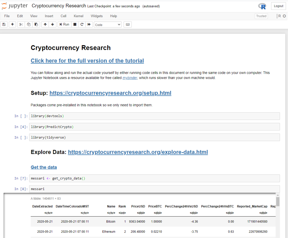
This can take up to 30 seconds to load, and once it has you should see a page that looks like this:

From here, you can run the code one cell at a time:

You can also use Shift + Enter to run an individual code cell
Or run all code cells at once:

If you feel lost and are not familiar with Jupyter Notebooks, you can do a quick interactive walkthrough under Help –> User Interface Tour:

2.2 Option 2 - Run Locally
If you want to follow along from your own computer directly (recommended option), please follow the installation instructions below. Afterwards, you will be able to run the code. You only need to follow these instructions once. If you have followed these steps once already, skip ahead to the next section.
2.2.1 Setup R
If you do not already have R and R Studio installed on your computer, you will need to:

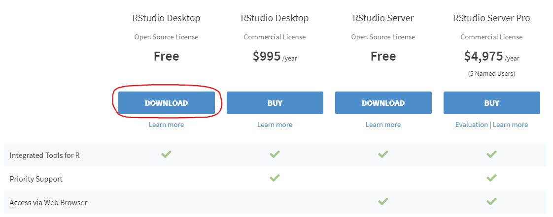
- Install RStudio. This step is optional, but it is very recommended that you use an integrated development environment (IDE) like RStudio as you follow along, rather than just using the R console as it was installed in step 1 above.

- Once RStudio is installed, run the application on your computer and you are ready to run the code as it is shown below and in the rest of this document!
You can run your code directly through the Console (what you are prompted to write code into when RStudio boots up), or create a new document to save your code as you go along:
You will then be able to save your document with the .R extension on your computer and re-run your code line by line.
2.2.2 Install and Load Packages
Packages are collections of functions and data that other users have made shareable outside of the functionality provided by the base functionality of R that comes pre-loaded every time a new session is started. We can install these packages into our own library of R tools and load them into our R session, which can enable us to write powerful code with minimal effort compared to writing the same code without the additional packages. Many packages are simply time savers for things we could do with the default/base functionality of R, but sometimes if we want to do something like make a static chart interactive when hovering over points on the chart, we are better off using a package someone already came up with rather than re-inventing the wheel for a difficult task.
2.2.3 Install Pacman
Let’s start by installing the pacman package (Rinker and Kurkiewicz 2019) using the function install.packages():
We only need to install any given package once on any given computer, kind of like installing an application (like RStudio or Google Chrome) once before being able to use it. When you boot-up your computer it doesn’t open every application you have installed and similarly here we choose what functionality we need for our current session by importing packages. All functionality that is made available at the start (foundational functions like mean() and max()) of an R session is referred to as Base R, functionality from other packages needs to be loaded using the library() function.
2.2.4 Load Pacman
We can load the pacman package using the library() function:
pacman does not refer to the videogame, and stands for package manager. After we importing this package, we can now use new functions that come with it.
2.2.5 Install All Other Packages
We can use p_load() to install the remaining packages we will need for the rest of the tutorial. The advantage to using the new function, is the installation will happen in a “smarter” way, where if you already have a package in your library, it will not be installed again.
p_load('pins', 'skimr', 'DT', 'httr', 'jsonlite', # Data Exploration
       'tidyverse', 'tsibble', 'anytime', # Data Prep
       'ggTimeSeries', 'gifski', 'av', 'magick', 'ggthemes', 'plotly', # Visualization
       'ggpubr', 'ggforce', 'gganimate', 'transformr', # Visualization continued
       'caret', 'doParallel', 'parallel', 'xgboost', # Predictive Modeling
       'brnn', 'party', 'deepnet', 'elasticnet', 'pls',  # Predictive Modeling continued
       'hydroGOF', 'formattable', 'knitr') # Evaluate Model Performance
It is normal for this step to take a long time, as it will install every package you will need to follow along with the rest of the tutorial. The next time you run this command it would be much faster because it would skip installing the already installed packages.
Running p_load() is equivalent to running install.packages() on each of the packages listed (but only when they are not already installed on your computer), and then running library() for each package in quotes separated by commas to import the functionality from the package into the current R session. Both commands are wrapped inside the single function call to p_load(). We could run each command individually using base R and create our own logic to only install packages not currently installed, but we are better off using a package that has already been developed and scrutinized by many expert programmers; the same goes for complex statistical models, we don’t need to create things from scratch if we understand how to properly use tools developed by the open source community. Open source tools have become particularly good in recent years and can be used for any kind of work, including commercial work, most large corporations have started using open source tools available through R and Python.
Nice work! Now you have everything you need to follow along with this example ➡️.
References
Rinker, Tyler, and Dason Kurkiewicz. 2019. Pacman: Package Management Tool. https://github.com/trinker/pacman.